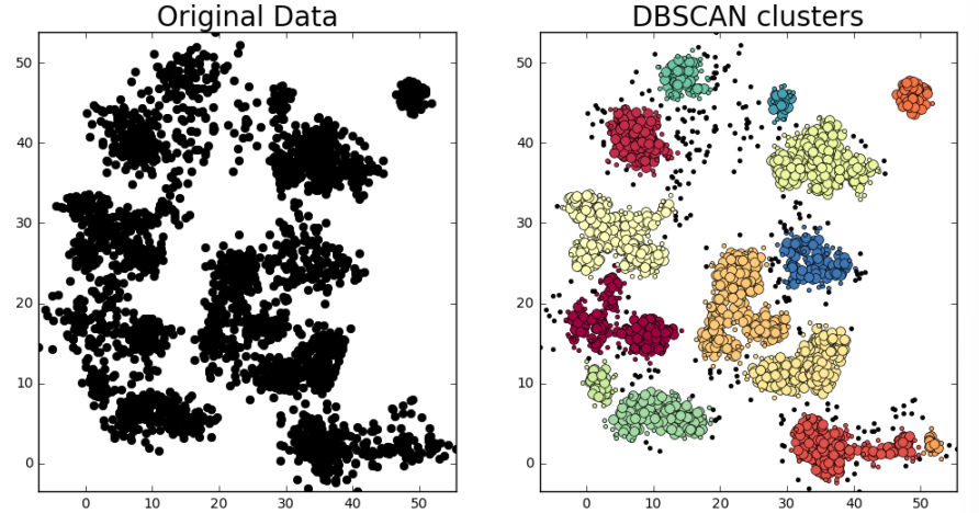
Clustering Analysis
Explores clustering types (partitional vs. hierarchical), cluster definitions (well-separated, center-based, density-based), and key algorithms including agglomerative hierarchical clustering, K-Means, and DBSCAN.
The purpose of clustering analysis is to find groups of objects which are related to each other. The definition of a cluster can be ambiguous, as we need to define what we consider a cluster.
Types of clustering
There are two kinds of clustering:
- Partitional clustering, it's the division of data into non overlapping clusters, so that a single data object is only in one subset
- Hierarchical clustering, the set of nested clusters which are organized in a hierarchical tree
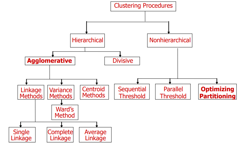 we can then also specialize the clusters into:
- Well-centered clusters
- Center-based clusters
- Contiguous clusters
- Density-based clusters
- Property or Conceptual
- Described by an objective function
Well-Separated cluster
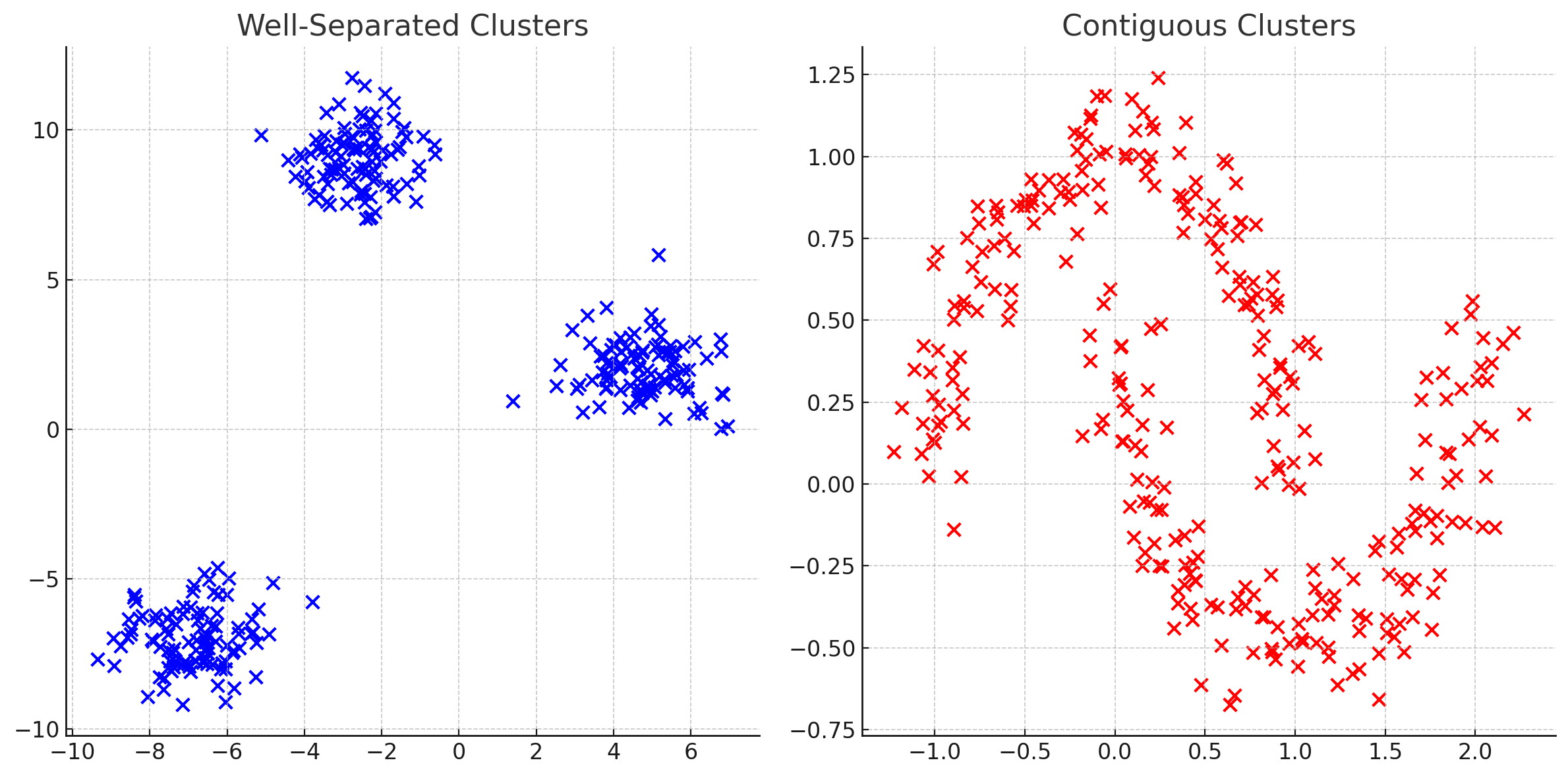
In the Well-separated cluster, a cluster is a set of points such that any point in cluster is closer (or more similar) to every other point in the cluster, than to any other point not in the cluster
Center-based cluster
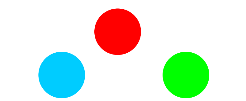
In the center-based cluster, a cluster is a set of objects such that an object in a cluster is closer (or more similar) to the "center" of it's cluster, than it is to the center of any other cluster. The center of the cluster is called centroid and it is the average of all points in the cluster, or alternatively, we use the medoid which is the point that is most "representative" of the cluster
Contiguity-based cluster
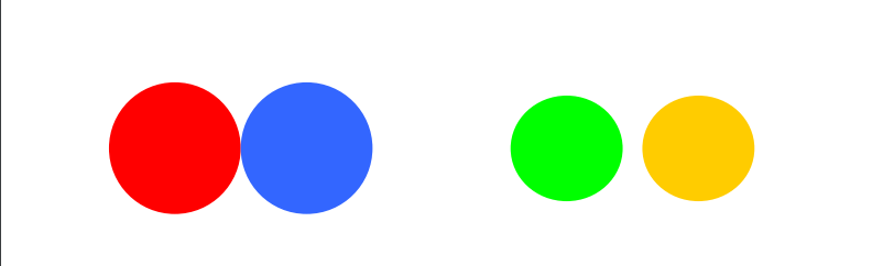
In the contiguity-based cluster, a cluster is a set of points such that a point in a cluster is closer (or more similar) to one or more points in the cluster than to any other point not in the cluster
Density-based clusters
In density-based clusters, a cluster is a dense region of points, which are separated by low density regions, and then again higher density regions. It is mostly used when clusters are irregular and intertwined, and when noise and outliers are present

Conceptual clusters
In conceptual clusters, a cluster is a set of objects that share a common propriety or particular concept (sub-space)

Hierarchical clustering
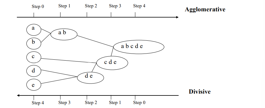
This is a typical clustering analysis approach which partitions data set sequentially. It constructs nested partitions layer by layer via grouping objects in a tree of clusters.
There are two approaches when building hierarchical clusters:
- Agglomerative, a bottom up strategy where initially, each data object is it's own atomic cluster, then we merge those clusters into larger and larger clusters
- Divisive, is a top down strategy where initially, all objects are in a single cluster, and we try to subdivide them into smaller and smaller clusters
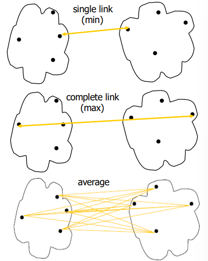
 There are also different methods to compare the distance between clusters:
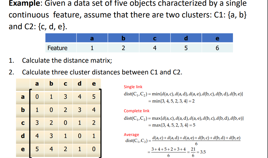
- Single link: the smallest distance between an element in one cluster and an element in another cluster.
- Complete link: the largest distance between an element in one cluster and an element in another cluster.
- Average: the average distance between elements in one cluster and elements in another.
Agglomerative Algorithm
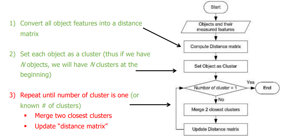
Agglomerative algorithm example:
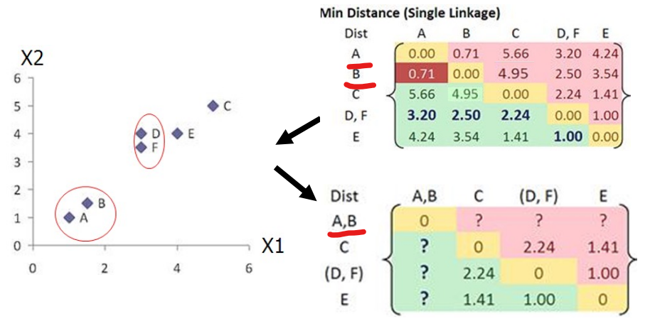
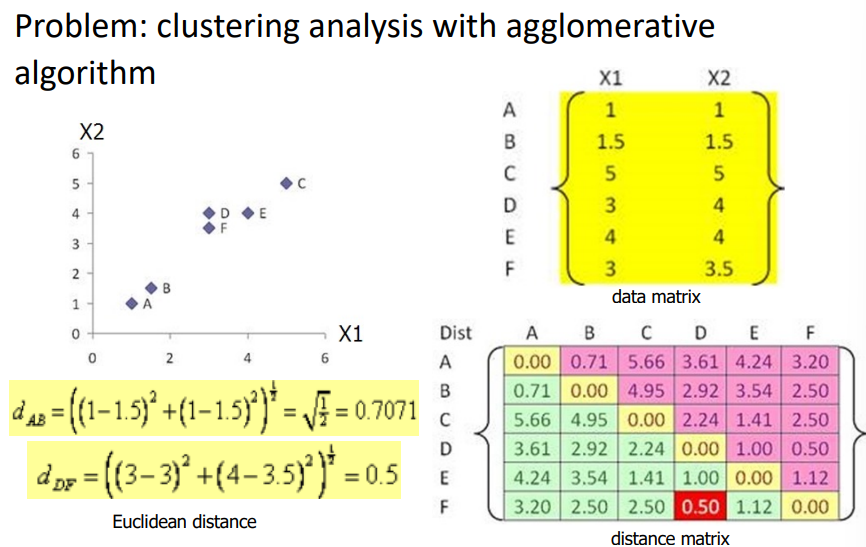 (Iteration 1) Merge two closest clusters
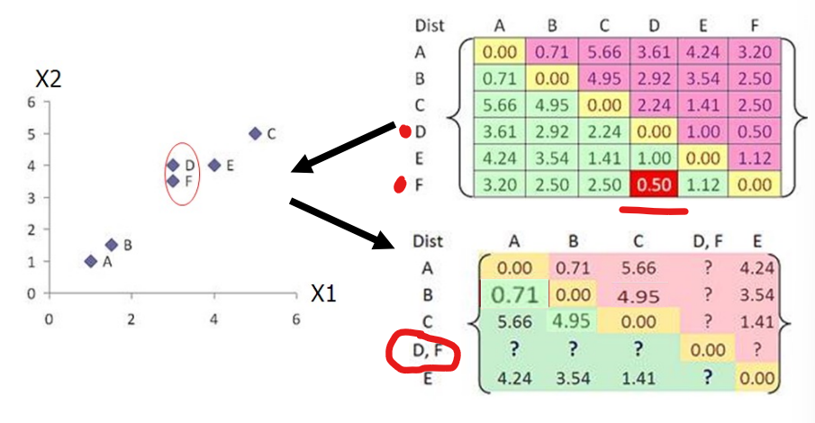 (Iteration 1) Update the distance matrix with the now merged D,F cluster
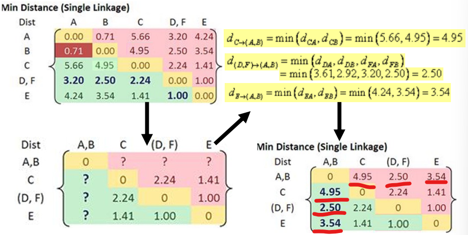
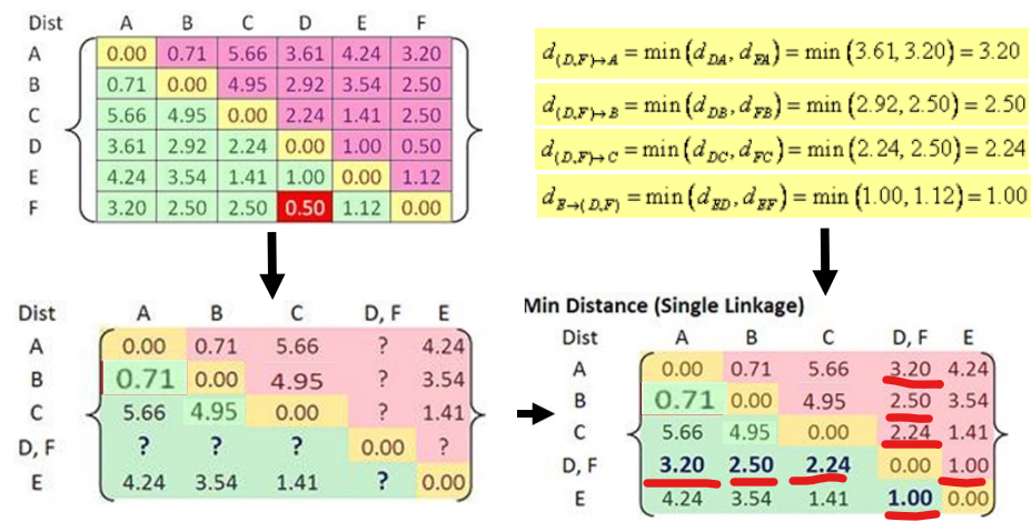 (Iteration 2) Merge the two closest clusters
 (Iteration 2) Update the distance matrix
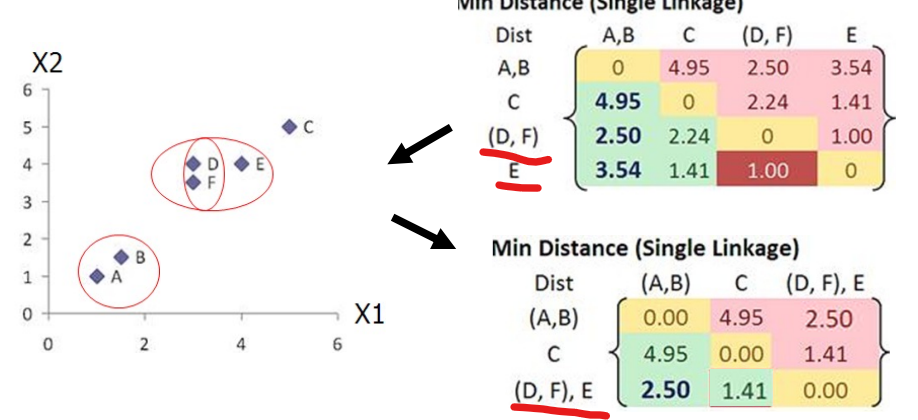
 (Iteration 3) Merge two closest clusters and update distance matrix
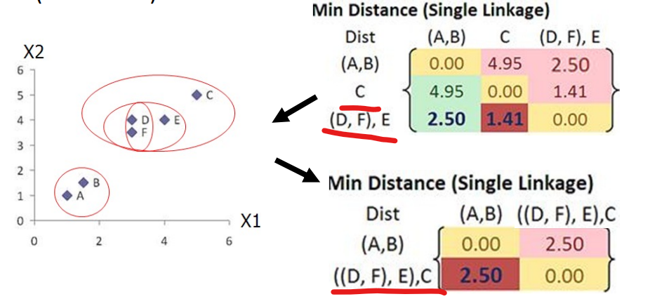
 (Iteration 4) Merge two clusters and update distance matrix
 (Iteration 5) Final iteration, merge the last two clusters, termination condition
We construct the Dendrogram tree of the cluster
(Iteration 5) Final iteration, merge the last two clusters, termination condition
We construct the Dendrogram tree of the cluster
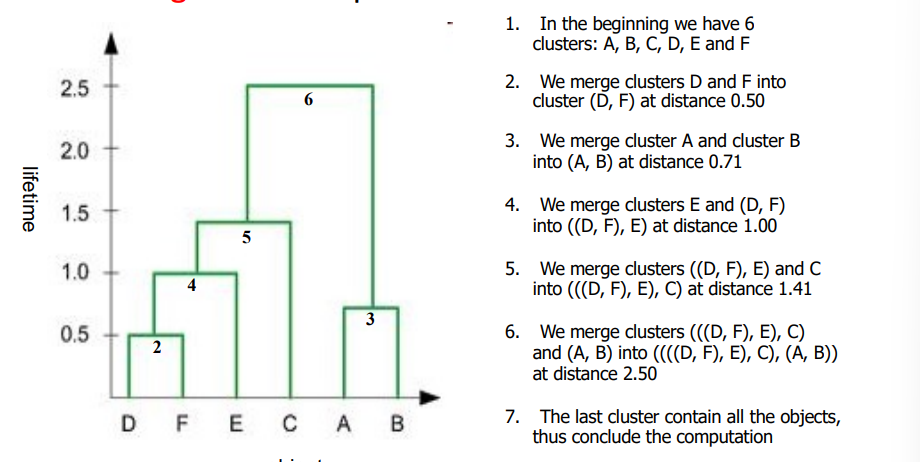
- The Lifetime of a cluster, as the difference between the proximity level moment the cluster was created, and the proximity level of when it was merged with any of the other clusters.
Taking the example of before: the lifetime of A, B, C, D, E, F are: 0.71, 0.71, 1.41, 0.50, 1.00, 0.50, and the lifetime of (A,B) is - The K-cluster lifetime is the distance from that K clusters merge to that of K clusters vanish due to the reduction to k-1 clusters
K-Mean clustering
link to demo Given a , find a partition of clusters to optimize the chosen partition criterion, in respect to a cost function. The -means algorithm is a heuristic method where each cluster is represented by the center of the cluster and the algorithm converges to stable centroids of clusters. It is the simplest and most used clustering analysis algorithm. It works by:
- Set centroids points randomly
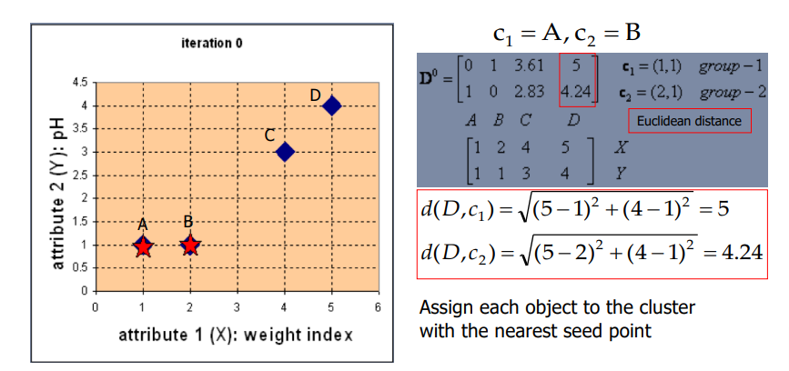
- Assign each object to the cluster of the nearest seed point measured with a specific distance metric
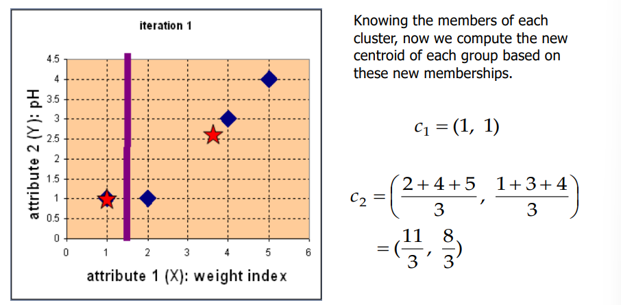
- Compute new centroids points of the current partition
- GOTO step 1, stop when there is no more new assignment, so each clusters does not change This algorithm has a computational complexity of where n is the number of objects, K is the number of clusters, and t is the number of iterations
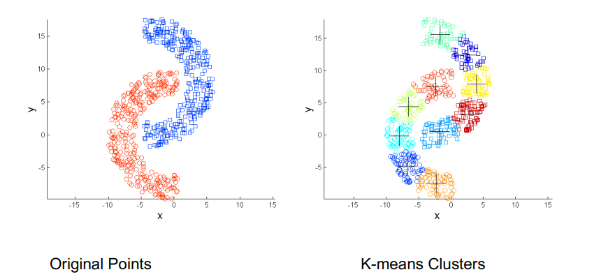
The problem with this algorithm is that it is sensitive to the initial seed points, and could fall into an unwanted local optimum. It also has the drawback of having to specify the number of clusters in advance, it can't handle (properly) noisy data and it is not suitable for clustering with non convex shapes. It is applicable only when the centroids are "definable"
Choosing the initial centroids
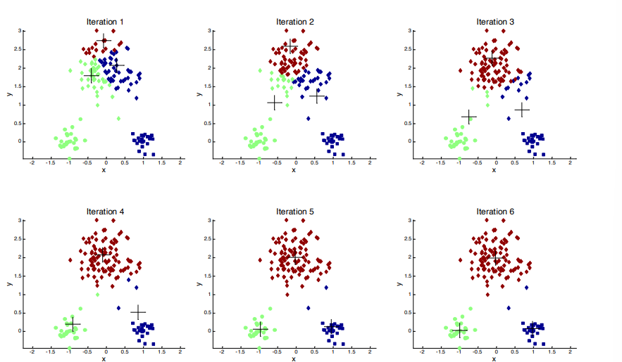
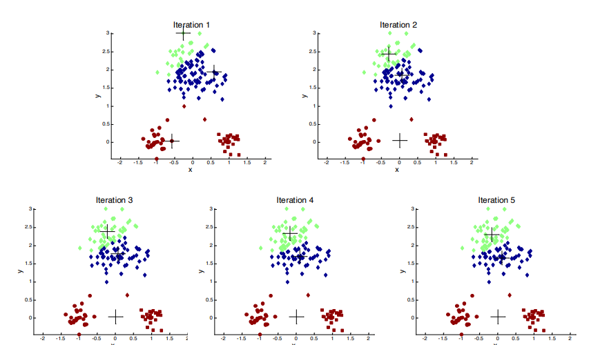
The chance of selecting one centroid from each cluster is really small, considering clusters of the same size then the probability of this is:
which even for K = 10, the probability is 0.00036. Sometimes the centroids will readjust themselves, other times they wont.
This is an example of a good first centroid choice
 While this is a bad example for the first centroid
 There are ways to mitigate this, such as:
- Using multiple runs, but the probability is not that much higher
- Use hierarchical clustering to determine the initial centroids
- Select more than initial centroids and then select the most widely separated ones, and apply some post processing to merge clusters together
K-Means limitations
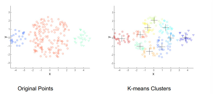
Differing sizes
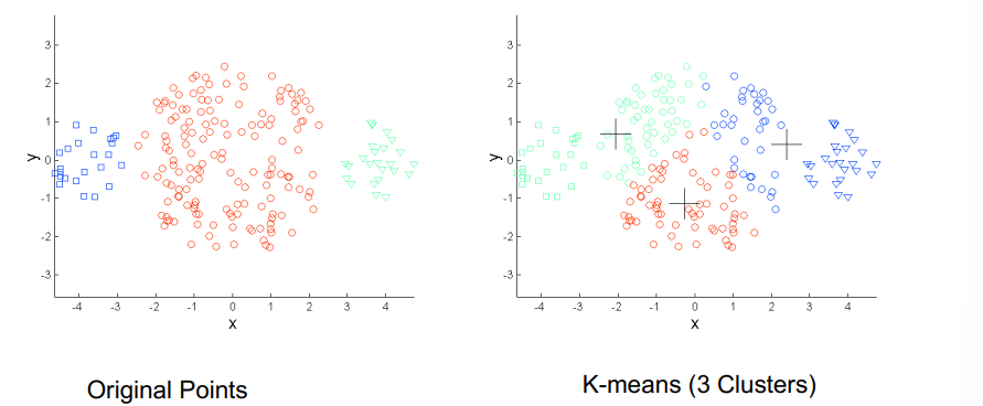 Can be solved by using more k-means clusters and then merging them
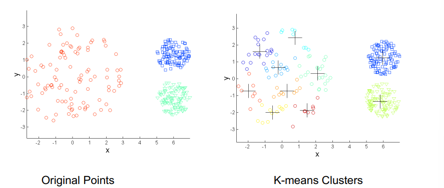
Differing density
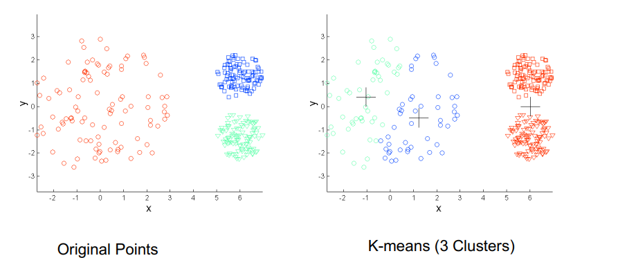 Can be solved by using more k-means clusters and merging them
Non globular shapes
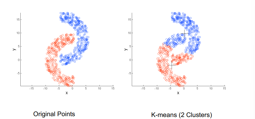 Can be solved by using more k-means clusters and merging them
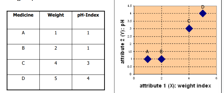
K-means example
Suppose we have 4 kinds of medicines, each has two attributes (PH and weight index), our goal is to group those objects into K=2 groups of medicines. We start off with this data set:
- Use initial seed points for partitioning
- Compute new centroids based off the current partitions
 Now modify the new membership of items based off the new centroids
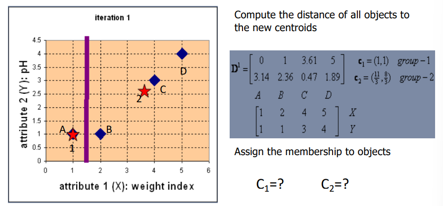
- Repeat the first two steps until its convergence
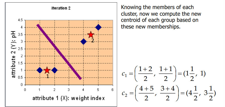
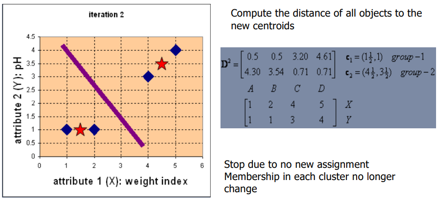
DB-Scan
link to demo It is a Density Based Clustering algorithm. It needs two parameters:
- to decide the size of the circle of each point whose nearby nodes are to be considered neighbors
- which is the minimum number of points to consider a point as a point During the execution, points are labeled in one of three types:
- Core points: those are the points which have at least of points inside of it's radius
- Boarder points: those are nodes which have a core point as neighbor but doesn't have enough neighbors to surpass the requirement
- Noise points: are points that don't have any neighbors
It executes by finding the first core points and then propagating the classification
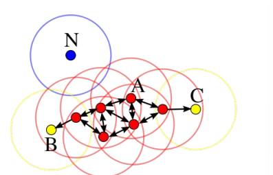 It has the advantage of:
- not requiring the number of clusters
- Can find any arbitrarily shaped clusters, even ones that are englobed by different clusters
- It is robust against outliers
- It is designed to be used in databases using R* trees
And disadvantages of:
- It is not deterministic, a border point which is reachable from more than one cluster could be part of either, depending in which order the data is processed
- The quality of the DBScan is dependent on the distance measure
- It is not very good at clustering data sets with large differences in density