Data is considered an anomaly if it does not conform to the expected behavior, they are also called outliers, exceptions, peculiarities etc... Examples of anomaly detection is credit card fraud, where a transaction looks unusual, or cyber intrusions where the network traffic is unusual

This is an example of possible outliers

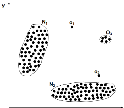
The key challenges for anomaly detection are:

• Defining the boundary of what is the normal region, and this is also often not precise
• The notion of outlier is different in each domain, so it is hard to generalize
• Availability of labelled data for validation and training of the model
• Data might contain noise
• Normal behavior keeps evolving

The most common data handled by anomaly detection is tabular data with binary, categorical, continuous and hybrid attributes.

There are three kinds of anomaly detection:

• Supervised anomaly detection: Labels are available for both normal data and anomalies
• Semi supervised anomaly detection: Labels are available only for normal data
• Unsupervised anomaly detection: No labels are provided, it is based on the assumption that anomalies are very different compared to normal data And also three kinds of anomalies:
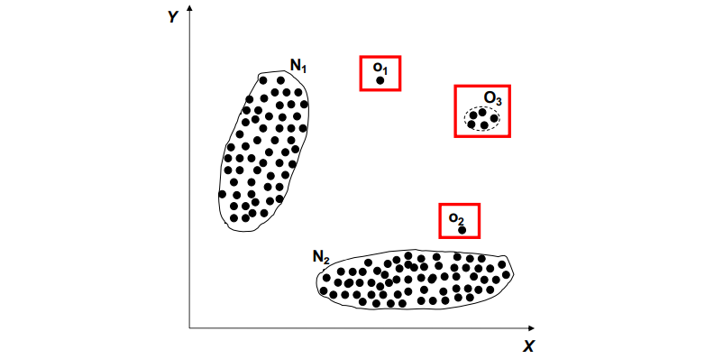
• Point anomalies: An individual data instance is anomalous
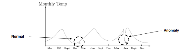
• Contextual anomalies: a data point is considered an outlier if it's value is significantly different from data points of the same context
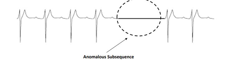
• Collective anomalies: a group of instances whose behavior is anomalous compared to other groups of instances

Point anomalies

Contextual anomalies

An individual data point is considered an anomaly depending on it's context. It requires the notion of the context it lies in, also called conditional anomalies

Collective Anomalies

A collection of data instances can also be called anomalous. It requires a notion of relationship between data instances. The individual instances within an anomaly are not anomalous by themselves, but together form an anomality

[excalidraw: Drawing 2025-04-09 12.08.27.excalidraw]

Outputs of Anomaly detection

Anomaly detection algorithms can output two kinds of data:

• Label: it is usually a boolean value, where each instance is given a normal or abnormal label. Especially useful in classification-based approaches
• Score: each instance is given a anomaly score, which gives more information, because in this way, outputs can be ranked, but to consider a point anomalous, we need a "threshold" or criteria to transform this numerical information into the anomalous or non anomalous label

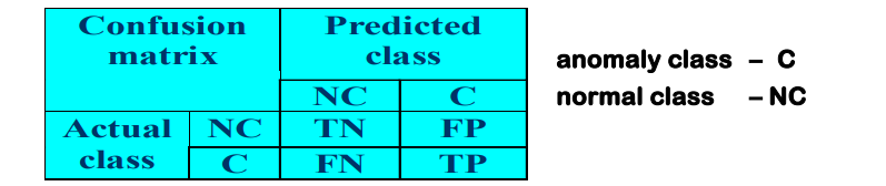
Accuracy on it's own is not able to judge the quality of a anomaly detection algorithm, as we could have a data set with 99.999% non anomalous values, and always return the non anomalous label for every data point. This algorithm would still be 99.999% accurate. Instead, we use the notion of false positive and false negative for both non anomalous and anomalous values, then use two metrics:

• Recall (R): $\dfrac{TP}{TP + FN}$
• Precision (P): $\dfrac{TP}{TP + FP}$ then combine the two into the $F{-}Measure = \dfrac{2RP}{R + P}$

Examples of known anomaly detection problems

Intrusion detection

It is the process of monitoring events in a computer system or network and analyzing them for intrusions, which are the attempts of bypassing the security mechanisms of a computer network.

The challenges of this is that most detection methods use signature based detection, which uses known patterns to determine an intrusion, and cannot detect new emerging threats.

Fraud detection

Fraud detection refers to the detection of criminal activities in commercial organizations, like a thief trying to use the payment method of a customer.

The challenges are to have a fast and accurate real time detection, where the misclassification cost is very high

Healthcare

Healthcare detection, detects anomalous patient records, that indicate a disease outbreak, instrumentation error etc.

The challenges are that only normal labels are available, and misclassification cost is very high. Data can be spatio-temporal

Image processing

Image processing is finding unusual behavior in a image that evolves overtime (security cameras). The key challenges is to detect collective anomalies, and data sets being really large

Classification based techniques

The classification based techniques are the ones that label the data as anomalous and not anomalous based off labeled training data, which then classifies new unseen events. They should be able to handle skewed/imbalanced class distributions

• Supervised: requires knowledge about both normal and anomaly classes, which are used to build a classifier that distinguishes normal and anomalies
• Semi-supervised: requires knowledge of normal class only, which are used to train a model that detects variations from normal behavior as anomalies The classification based techniques have advantages and disadvantages such as:

Supervised classification techniques: the models can be easily understood and have high accuracy in detecting many kinds of KNOWN anomalies, but they cannot detect UNKNOWN and emerging anomalies. Having labels for both normal and abnormal data might be difficult Semi-supervised classification techniques: the models can be easily understood and have high accuracy in detecting normal behavior, but they could possibly have high false alarm rate for previously unseen normal records that might be recognized as anomalies

Manipulating data records

There might be way more normal records (Majority class) than anomalies (Rare class) in our data, and we want to be able to train a model that recognizes them. For this reason we might want to manipulate our data records to more effectively create a recognition model

• Over sampling the rare class: Make duplicates of rare events until the data set contains as many samples as the majority class. This does not increase information but increases misclassification cost
• Generating artificial anomalies: SMOTE (Synthetic Minority Over-sampling TEchnique): new points of the rare data are generated in regions of existing rare class examples, they are generated around the edges of sparsely populated data regions
• Down sizing (undersampling the majority class): Sample randomly the data records from the majority class and replace them with the whole majority class so that both rare and majority classes have the same number of records. This looses a high amount of information, and is not viable if the rare class is very small

Support vector machines (SVM)

It uses the idea that normal data belongs to high density regions, while anomalies are in low density regions. It separates the entire set of training data from the origin to find regions where most of the data lies, to then label this region as a class. When new data comes in, it is compared to the same space and predicted to belong to either one of the two categories based off which side of the gap they fall. It works by finding a hyperplane (which is often bigger than the original vector plane) where data lies in two separate regions.

Nearest Neighbors based techniques

For the NN techniques we make the assumption that: normal points have close neighbors while anomalies are located far apart from other points

The general approach is to compute the neighborhood for each data record and then analyze the neighborhood to determine which data record is an anomaly or not

There are both:

• Distance based techniques: anomalies are data points which are the most distant from other points
• Density based methods: anomalies are data points in low density regions

They have the advantage of possibly being either unsupervised or semi-supervised, but have the drawback of not being able to work very well in sparse data, and in high dimensional spaces, the concept of similarity loses effectiveness because of the curse of dimensionality, where the distance between each point might become very similar (small) and so each record might be considered an outlier/inlier

Distance based techniques

The point $O$ in a dataset $D$ is a $DistBasedFun(p,d)$ outlier, if at least a fraction $p$ of the points in the dataset lies at a distance further than $d$ from the point $O^*$. One such algorithm is the (K nearest neighbors) KNN algorithm:

• For each data point $d$ compute the distance to the $k^{th}$ nearest neighbor $d_k$ (find the nearest neighbor $n$ and then pick, from the $k$ nearest neighbors of $n$, the closest one)
• Sort all data points according to the distance $d_k$
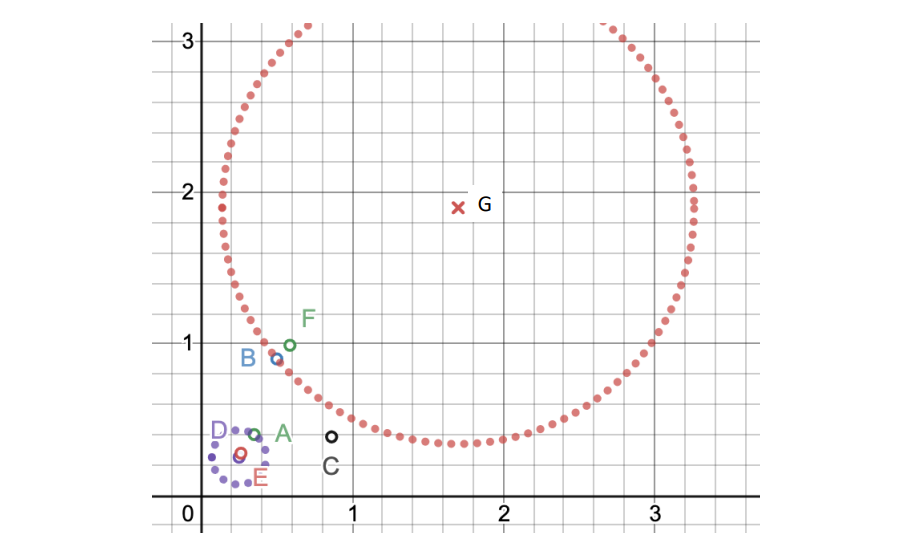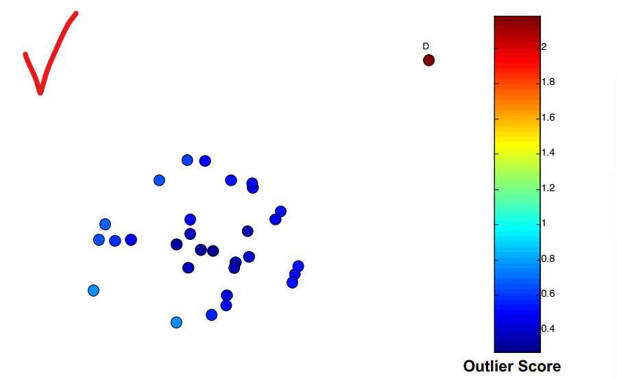
• Outliers are the points that have the highest distance $d_k$, and therefore located in the most spare neighborhoods The problem with this algorithm is finding a suitable $k$ because, let's set 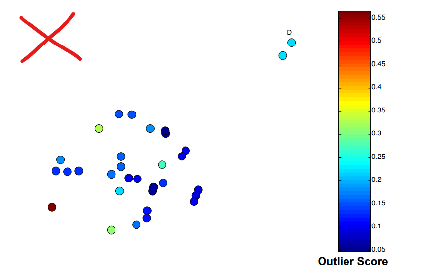$k = 1$ now let's set 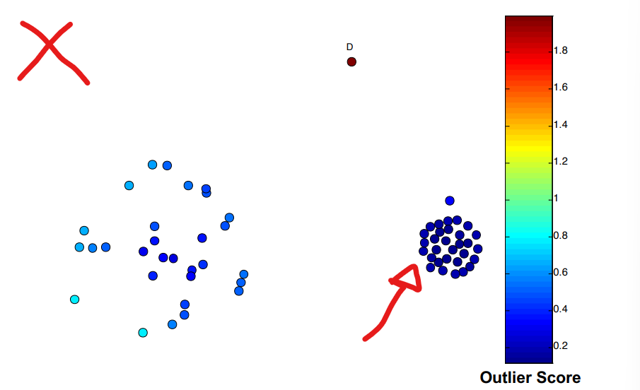$k = 5$ the group on the right is still an outlier, but is clustered up (at this point, since the significance of the cluster, should this even be considered an outlier?)

Local Outlier Factor (LOF)

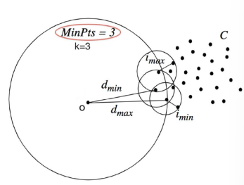
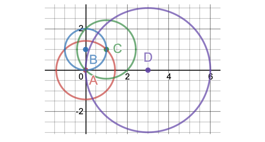
k-th Nearest Neighbor Distance (k_dist): The k-th nearest neighbor distance of a point $p$, denoted as $k{\_}dist(p)$, is the distance between point $p$ and it's $k^{th}$ nearest neighbor

Reachability Distance (reach_dist): The reachability distance of two points $q$ and $p$, denoted as $reach{\_}dist_k(q,p)$ is defined as:

$$\Large reach{\_}dist_k(q,p) = max\left\{ k{\_}dist(q),\, d(q,p)\right\}$$

Local Reachability Density (lrd): The local reachability density of a point $q$, denoted as $lrd(q)$, measures how closely packed the $MinPts$ neighbors $N_{MinPts}(q)$ are to the point $q$, it is defined as:

$$\Large lrd(q) = \dfrac{MinPts}{\sum\limits_{p \in N_{MinPts}(q)}{reach\_dist_{MinPts}(q,p)}}$$

Local Outlier Factor (LOF): The local outlier factor of a point $q$, also denoted as $LOF(q)$, is the comparison between the local reachability density of a point $q$ with the local reachability densities of it's neighbors, it is defined as:

$$\Large LOF(q) = \dfrac{1}{MinPts} \cdot \sum\limits_{p \in N_{MinPts}(q)}{\dfrac{lrd(p)}{lrd(q)}}$$

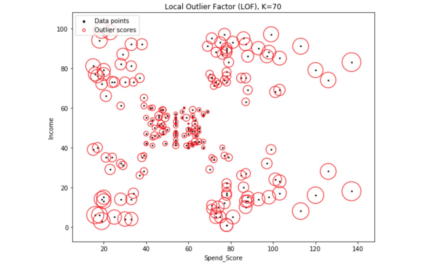
• if $LOF(q)$ is significantly greater than 1: $q$ can be considered an outlier, as it's local density is much smaller than it's neighbors, whereas
• if LOF(q) is close to 1 or smaller: $q$ can be considered an $inlier$ as it's part of a dense area

Advantages of LOF compared to K-NN

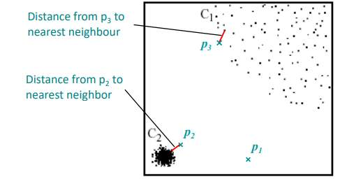In the K-NN approach, $p_2$ will not be considered an outlier, but the $LOF$ approach will consider both $p_2$ and $p_1$ as outliers. In a sparse area, the K-NN approach might consider the point $p_3$ as an outlier, but the $LOF$ approach does not, as the local density of $p_3$ is similar to it's neighbors