
Similarity and Distances
Defines and compares distance and similarity functions for quantitative, categorical, text, binary, time-series, and graph data, including Lp-norms, the curse of dimensionality, cosine similarity, Jaccard coefficient, DTW, and graph kernels.
Many data minding problems, such as clustering, outlier detection and classification require the computation of similarity DEFINITION Given two objects and , we want to compute the similarity or distance , between the two objects.
In similarity functions, a high value means greater similarity, while in distance functions, smaller values imply greater similarity. Depending on the domain, it makes more sense to talk about either distance or similarity
Distance functions are fundamental to the effective design of data mining algorithms, as a poor distance function could reduce the quality of the result drastically
Quantitative Data ()
The most common distance function is the , between two data points: and is defined as:
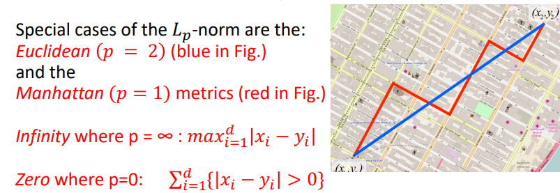
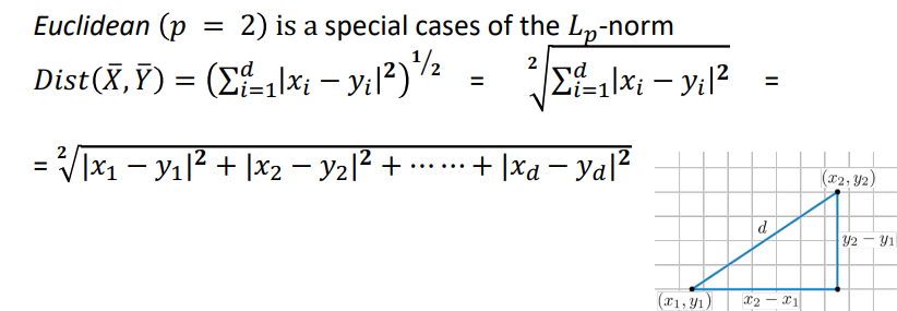 The euclidian distance is the "straight line" between two data points, it has a nice propriety of being rotation invariant, because the distance does not change if we rotate the axis system. This also means that the techniques like PCA, SVD and wavelet transformation for time series can be used without affecting the distance. In high dimensionality data, this function might not work very well because of the varying impact of the data sparsity, distribution, noise and feature relevance
Minkowski Distance
In some cases we know which features are more important than others, it is the same as the except we introduce a new coefficient that is associated with the feature, this coefficient is used to weight the feature
Impact of high dimensionality
Distance based data mining applications lose their effectiveness as the dimensionality of the data increases, this phenomenon is referred to as the curse of dimensionality.
Consider an unit cube of dimensionality that is fully located in the non negative quadrant, with one of the corners in the origin . What is the manhattan distance of the corner of this cube to a randomly chosen point inside the cube? in this case, as we are in the non negative quadrant and one point is in the origin, the manhattan distance will simply sum up all the coordinates of the point in the different dimensions. Each coordinate is uniformly distributed in
Therefore, if represents the uniformly distributed random variable in , the manhattan distance is as:
For large values of it can be shown that by the law of large numbers, the vast majority of randomly chosen points inside the cube, will lie in the range:
so the points in the cube will lie within a distance range from the origin of:
The ratio of the variation in the distance is referred to as and is given by:
This ratio can be interpreted as the distance contrast between the different data points, in terms of how different the minimum and maximum distances from the origin might be considered. The contrast reduces with which means there is virtually no contrast with increasing dimensionality. A low contrast value means that the mining algorithm will score the distances between all pairs of data approximately the same
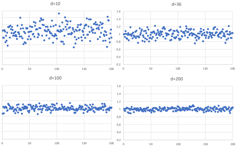 Causing the distance to become less meaningful
Match based similarity computation
High dimensionality data sets are often likely to contain diverse features, many of which are irrelevant. The subset selection during the preprocessing does not solve the problem, as the relevance of features is locally determined by the pair of objects that are considered.
Proximity thresholding
One way to de ephasize the levels of dissimilarity is by proximity thresholding in a dimensionalty-sensitive way, it works by:
- Each dimension is divided into equi-depth buckets (as in, there are the same number of instances in each bucket), containing of the records. The number of buckets depends on the data dimensionality
- let and be two points, then for each dimension , if both and belong in the same bucket, they are said to be in proximity on dimension
- The subset of dimensions in which and map to the same bucket is referred to as the Proximity set, containing all dimensions in which they are in proximity of. This set is called
- For each dimension , let and be the upper and lower bounds values of the bucket in dimension in which the two records are proximate to one another (imagine the dimension as a line, the m and n are the "ranges" in which the values lay)
The value of the expression will vary between 0 and because each individual expression in the summation lies in between 0 and 1. This is a similarity function because larger values imply greater similarity, and it guarantees nonzero similarity only for dimensions mapping to the same bucket By using the equi-depth partition, we ensure that the probability of two records being in the same bucket in a particular dimension is non zero components
Using Categorical data
If no ordering exists among the discrete values of categorical data, we can compute it by transforming the data to numeric data, using the binarization approach. For categorical data, it's more common to work with similarity, because discrete values can be matched more naturally
The simplest similarity function between and is the sum of the similarities of the individual attribute values. If is the similarity between the attributes of the values and , then the overall similarity can be defined as:
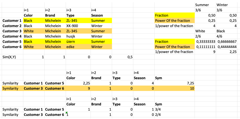
We now need to define function , the simplest is simply returning 1 if , otherwise return 0. This obviously doesn't account for the relative frequencies of the different attributes. Two records that have a "normal" value for this attribute do not provide significant information about the similarity, because the majority of pairs likely show that pattern by chance. The matches of a categorical attribute which have unusual values should be weighted more heavily than the ones that appear frequently. We call this the Inverse occurrence frequency, which weights matching attributes by the inverse function of the frequency of the matched value. So, when , the similarity is equal to the inverse weighted frequency, and otherwise
Let be the ratio (amount) of records in which the attribute has the value of in the data set, then we define as:
Goodall measure
Related to the previous measure, where the similarity of the attribute is defined as , so:
Mixed quantitative and categorical
To generalize the approach to mixed quantitative and categorical, we add weights based of the numeric and categorical components. The problem is deciding how to assign the weights. Consider two records: and where are the subsets of numerical attributes, and the subsets of categorical attributes, then the similarity between can be defined as:
The parameter regulates the importance of the categorical an numerical attributes, without any domain knowledge, we could assign the value of to the number of numerical attributes in the data. The proximity of Numerical data is often computed using distance function rather than similarity. In this case we can also convert the distance values to similarity values, for a distance value of , a common approach is to use a mapping that yields a similarity value of , or viceversa
Text similarity
When treating text as a bag of words (dictionary), then we can treat it as a quantitative mutidimensional data. we can consider:
- The frequency of each word can be treated as a quantitative attribute and the base lexicon can be treated as the full set of attributes
- Text is very sparse, so most attributes take the value of 0
- All the frequencies are non negative
- Measures like the -norm do not work well to the varying of the length of different documents in the collection. (for example, the -distance between two long documents will always be larger than the one between two short documents, even if the two big documents have many words in common) We normalize the irregularities by using the cosine measure which computes the angle between two documents, which is insensitive to the length of the document
Let and be two documents of lexicon of size , then the cosine measure is defined as:
If two documents match on an uncommon word, then this is more indicative of similarity than the case in which two documents match on a word which occurs very commonly
The inverse document frequency which is the decreasing function of the number of documents in which the word occurs, is commonly use for normalization over documents, it calculates how common or rare the word is across documents
and a damping function , like the square root or the logarithm can be applied before the similarity computation:
Binary multi dimensional data
Binary multidimensional data are a representation of set based data where a value of indicates the presence of the element in the set. If and are two sets with binary representations and , then we can use the jaccard coefficient (which sees the number of common and disjoints elements in two sets)
or if we have a damping function:
Time series similarity
The design of the time-series similarity are very application specific, we need to consider:
- Behavioral attribute scaling and translation: different time series may not be drawn on the same scales. For example, the time series of stock values might have similar patterns, but with different absolute values, both in mean and standard deviation
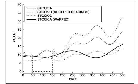
- Temporal (contextual) attribute translation: in some applications, the ABSOLUTE timestamp is not important, in those cases the temporal attribute value need to be shifted in at least one of the time series to allow for a more effective matching
- Temporal (contextual) attribute scaling: the series may need to be stretched or compressed along the temporal axis to allow for more effective matching. This is also called time warping
- Non contiguity in matching: long time series may have noisy segments that don't match with one another. The distance function needs to be able to handle such noise, alternatively, those issues can be addressed by attribute normalization during preprocessing
DTW Distance
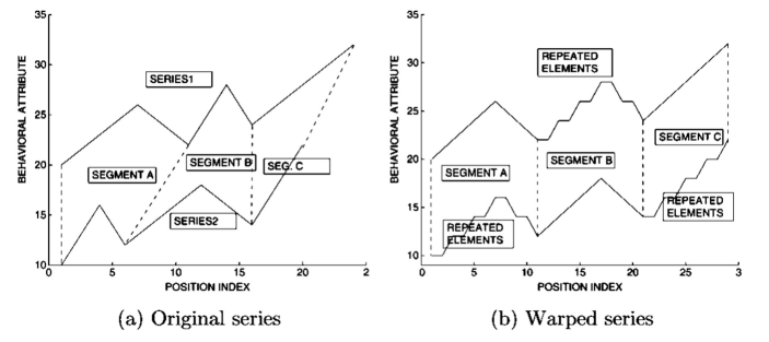
the DTW (dynamic time warping distance) stretches the series along the time axis, in a dynamic way, over the different portions, to enable better matching link to the algorithm
an example usage is for speech recognition, where words might be spoken in a different speed
Discrete sequence similarity measures
The edit distance (or levenshtein distance) is the distance between two strings, as the least amount of "effort" required to transform one sequence into another, by a series of transformations called "edits", which can be either: insertion, deletion, replacement. Example, consider the two strings:
ababababab bababababa
on the alphabet {a,b}, we can transform it either by:
- transforming every symbol of the other string (cost 10)
- delete the leftmost element of the string and inserting the "a" as the rightmost element (cost 2)
Longest common sequences (LCSS)
Consider the two strings:
agbfcgdhei afbdgchdei
in this case, "ei" is a substring of both sequences, but also a subsequence. "abcde" and "fgi" are also subsequences, but not substrings.
- Subsequences of longer length are indicative of a greater level of matching between the strings
- The length of the longest common subsequence (LCSS) is a similarity function, because higher values indicate higher similarity
Graph similarity measures
We can consider the similarity in graphs related to two graphs or between two nodes in a single graph
let be an undirected network with nodes set and edge set , where costs or weights are associated with edges
- the distance functions work with costs, whereas similarity functions work with weights. we consider the cost and the weight of the edge
- the principle of similarity between two nodes are based odd the concept of homophily where nodes are typically more similar in a network when they are connected to one another with edges. Nodes that are connected with shorter paths, or many paths, should be considered similar
Structural Distance-Based Measure
let the shortest path between node to any node , the value of is initialize to 0 for and otherwise. then we use the Dijkstra algorithm to find the shortest path
Random walk-based similarity
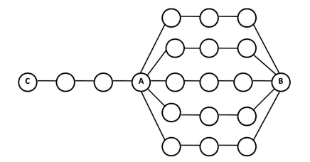 in this graph, the shortest path between and is 3, and the distance between and is 4, yet, we should consider the node as being more similar, because for the , node and share more paths
the intuition is: if you were lost in a road network and drove randomly, taking turns (joints) randomly, which location are you more likely to reach?
starting from node a we are more likely to end up in rather than
in this graph, the shortest path between and is 3, and the distance between and is 4, yet, we should consider the node as being more similar, because for the , node and share more paths
the intuition is: if you were lost in a road network and drove randomly, taking turns (joints) randomly, which location are you more likely to reach?
starting from node a we are more likely to end up in rather than
Similarity between two graphs
Determining the similarity between two graphs is extremely hard (NP-hard), core ideas to compute it are:
- Maximum common subgraph distance: When two graphs contain a large sub-graph in common, then they are considered similar
- Substructure-based similarity: It is difficult to match two large graphs, in alternative we match smaller substructures instead
- Graph-edit distance: The distance measure is analogous to the string edit distance, it counts the number of edits to transform one graph to the other
- Graph kernels: shortest path kernel and random walk kernel