What is data mining

Data mining is the study of:

• Collecting
• Cleaning
• Processing
• Analysing
• Gaining insight from data

Data mining categories

Data mining is a broad term that collects different kinds of data manipulation and analysis, each problem might be drastically different to solve compared to the rest, but they fall under those 4 categories

• Association pattern matching
• Clustering
• Classification
• Outlier detection

These are the building blocks over which applications are built upon. It is also used as an abstraction to help us conceptualize and structure data

Data mining process

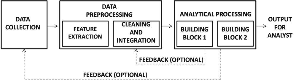
Data collection

it may require the use of hardware such as sensors, manual labor through user surveys, software tools to scrape data, etc...

Data processing

As we saw through the data collection, this data can come from different sources and be of different encoding, this step converts arbitrary data into a single format that is friendly to data mining algorithms

This comes with the problem that missing or erroneous information is present in the data. In the process of feature extraction, missing data should be estimated and erroneous data corrected. What features to extract from data depend on how relevant they are with the particular application we are analyzing and needs experience to filter correctly. Introducing unnecessary features might slow down the processing, while leaving some out might lead to incorrect analysis.

Some input data might be erroneous or missing, causing the whole data entry to be either dropped or modified to fit the dataset, for example we expect a feature containing the age to be between 0 and 100

Analytical processing

The final stage uses the processed data to run the analytical methods that will be used to find what we need from the data. In many cases it's not possible to use directly one of the building blocks (the macro categories), but an application can be split into multiple ones to find a solution to an application.

Data types

Data can also fall under different domains, we classify them under:

• Quantitative (e.g. age, height, ...)
• Categorical (e.g. Colour)
• Text
• Spatial
• Temporal
• Graph oriented The most common data type is multidimentional, joining different data types

Multi dimensional data

A multidimensional dataset D is a set of $n$ records $X_1,...,X_n$ such that each record $X_i$ contains a set of features denoted as $x_i^1,...x_i^d$

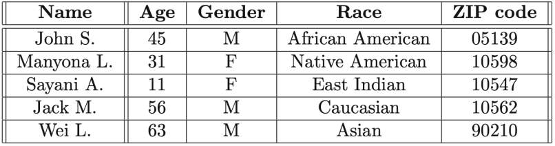
• An attribute is called quantitative if it has a natural ordering, also called continuous, numeric or quantitative. This is the most common subtype of data and is easy to work with in a statistical perspective, (e.g. age)
• An attribute is called categorical or Mixed attribute if it's part of a discrete set without a natural ordering among them, (e.g. gender, race, zip code)
• An attribute is called binary if it has only two possible values, it could be considered either a categorical or quantitative data type. It is also used as a set element indicator to represent setwise data, to specify if an element should be included in the set or not
• Text attributes are treated differently as they are not very useful when represented in it's raw form of text strings, in practice, a vector space representation is used, where the text can be considered a multidimensional quantitative data, where each attribute is a word/term, and the values correspond to the frequencies of these attributes. Frequencies are often normalized based off the length of the document and all the different terms in the document. The corresponding matrix is a $n\times d$ data matrix for a text collection with n documents and d unique terms (also known as vocabulary)

Dependencies in data

Data can also be either:

• Non Dependency oriented (NOD): the data records don't have any dependencies among other data or attributes, for example a person's name, gender, etc
• Dependency oriented (DO): Implicit or explicit relations may exist between data items

Dependency oriented data

Data values may be related to each other temporally, spatially or with explicit network relationships. The knowledge of existing dependencies can change the data mining process, and dependencies can be of type:

• Implicit dependency: the dependencies between data are not explicit but are known to typically exist in that domain, (e.g. that consecutive values of a temperature sensor are similar to each other and don't vary greatly between single readings)
• Explicit dependencies: it refers typically to graph or network data where edges are used to define explicitly the relationships between data

DOD: Time series data

Time series data contain values that are generated by a continuous measurement over time, like a temperature sensor or ecg, they have usually implicit dependencies between values over time. To extract those dependencies, we define two kinds of attributes:

• Contextual attributes: They define the context on the basis of which the implicit dependencies occur in the data, for example the timestamp in a sensor reading might be considered a contextual attribute, and time series data contain only one contextual attribute
• Behavioural attributes: They represent the values that are measured in a particular context, for example, in a temperature reading, the context is the timestamp and the actual temperature is the behavioural attribute DEFINITION A time series of length $n$ and dimensionality $d$, contains $d$ numeric features at each of $n$ timestamp $t_1,...,t_n$. where the values received at timestamp $t_i$ is $Y_i = (y_i^1,...,y_i^d)$ and the $j^{th}$ value of a series at timestamp $t_i$ is $y_i^j$.

DOD: Discrete sequences and strings

A discrete series is a stream of actions that happen in order, it can be an analogy of time series, where the contextual attribute is a timestamp, or position index of when the attribute appeared in the sequence. DEFINITION A discrete sequence of length $n$ and dimensionality $d$ contains $d$ discrete feature values at each of $n$ different time stamps $t_1,...,t_n$. Each of the $n$ components $Y_i$ contains $d$ discrete behavioral attributes $(y_i^1,...,y_i^d)$, collected at the $i^{th}$ time-stamp.

DOD: Spatial and Spatiotemporal

• In spatial data, many non spatial attributes (e.g. temperature, pressure, etc) are measured at a specific spatial location. In this case spatial coordinates correspond to contextual attributes, whereas the other attributes like temperature, pressure etc, are considered behavioural attributes
• Spatiotemporal data contains both spatial and temporal attributes, and two different kinds of spatiotemporal data exist:
  • Both spatial and temporal attributes are contextual: is a generalization of spatial and temporal data, it is useful when the behavioural attributes are measured simultaneously.
  • The temporal attribute is contextual and spatial attributes are behavioural: This can also be considered a time series data, but the spatial nature of the attributes can help in the interpretation of the data and improve the analysis on many scenarios

DOD: Network and Graph Data

In a network and graph data, the values of data are represented as nodes/vertices and the relationships among them are represented through edges/links in the network. Attributes cna bee associated to both nodes and edges in the network. DEFINITON A network $G = (V, E)$ contains a set of nodes $V$ and a set of edges $A$ where the edges in $A$ represent the relationships among nodes (the edge can be directed or undirected). An attribute set $X_i$ may be associated with node $i$, an attribute $Y_{ij}$ may be associated with edge $(i,j)$

An example of a network is a social network, where nodes represent people and edges their friendship links, each node may have attributes like their social media content

Kinds of relationships

Relationships in data items are of two kinds:

• Relationship between columns(attributes): There are frequent or infrequent relationships between values in a row, aka, positive or negative association pattern mining problem. One particular column is considered a target and it is used to direct the data mining process of the application specific way. This is also called supervised data mining. It is used to determine the relationship and predict a target value (classification)
• Relationship between rows(records): The goal is to determine a subset of rows in which the values of the columns are related to each other, if these subsets are similar, we call them clustering. If some rows are very different from all the rest, those are called anomalies/outliers, referred to the outlier analysis.

Association pattern matching

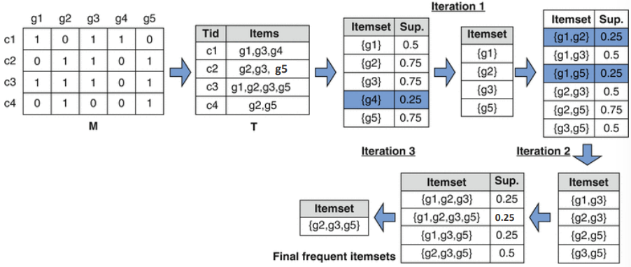
It is a problem defined over sparse binary databases, where values are either 0/1 and most of the values are 0. An example is a transaction in a shop, a record(row) in the matrix is a single transaction, and the columns(attributes) are if the transaction contains an item or not, formally, the $(i,j)^{th}$ entry is 1 if the transaction $i$ contains item $j$.

DEFINITION (Frequent pattern mining) Given a binary $n \times d$ data matrix $D$, determine all subsets of columns such that all the values in these columns take on the value of 1 for at least a fractions $s$ of the rows in the matrix. The relative frequency of a pattern is referred to as its support. The fraction s is referred to as the minimum support.

For example, if 3 columns are often all present in many records, it means that those items are probably bought together.

Data clustering

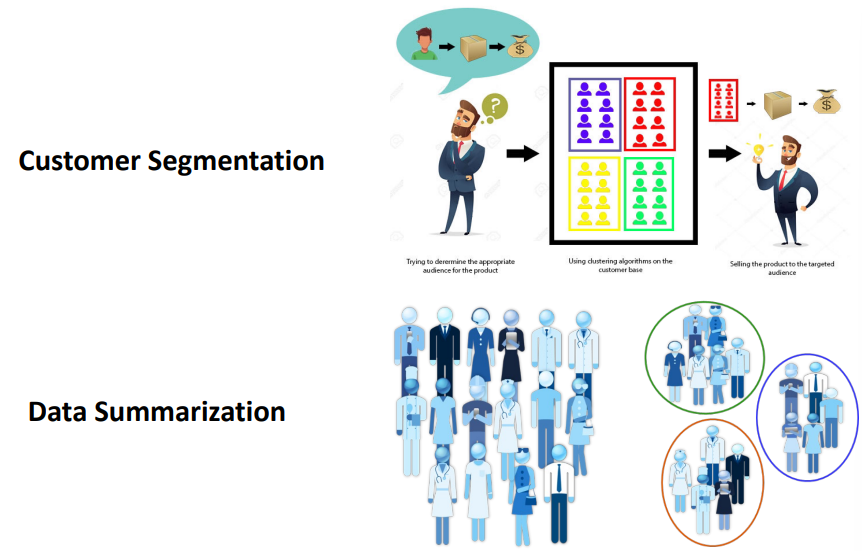
DEFINITION Given a data $n \times d$ data matrix $D$, partition its rows (records) into $k$ sets $C_1,...,C_k$ such that the rows (records) in each cluster are “similar” to one another. A clustering problem can be seen as a optimization problem where the variables of the optimization problem can represent the membership of of datapoints in a cluster, and a objective function that maximizes a quantification, or similarity in terms of those variables. An example of this is:

• Customer segmentation: determine the customers that are similar to one another
• Data summarization: clusters can be considered similar groups of records, groups can be seen as a summary of the data

Outlier detection

An outlier is a datapoint that is significantly different from the remaining data. "An outlier is an observation that deviates so much from the others as to arouse suspicion that it was generated by a different mechanism", they are also called abnormalities, deviants, anomalies. DEFINITION Given a data $x \times d$ matrix $D$, determine the rows of the data that are very different from the others in the matrix

The outlier detection is related to clustering as a complement, since in clustering we try to find the main groups, what's left out are the outliers

Outlier detection is useful in many different fields, like monitoring activity in a network or system to detect malicious activity, unusual spending for credit card frauds, sensor events, medical diagnosis, etc...

Data classification

Many data mining problems are directed towards a specialized goal that is sometimes encoded in a feature in the data. We have a starting data set called training data that we use to train a model, which is then used to predict class labels for records where the label is missing. For example, in a marketing application, a record might be tagged with a label that represents the interest of a consumer towards a product, and having a history of transactions we can guess what product they might be interested in.

DEFINITION Given an $n \times d$ training data matrix $D$ and a class label value in ${1,...,k}$ associated with each of the $n$ rows in $D$, create a training model $M$ which can be used to predict the class label of $y$, a $d$-dimensional record, where $y \notin D$

Relationship among problems

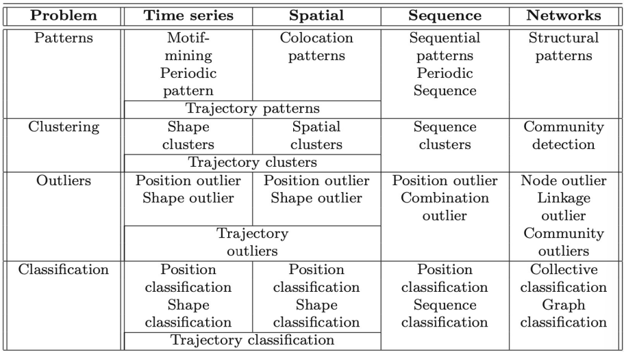
• In the clustering problem, the data are partitioned in k groups on the basis of similarity, we could view this as the "unsupervised" version of classification
• In the classification problem, a record is categorized into one of the k groups, but this is achieved by learning a model from a training database, we could view this as the "supervised" version of clustering

Scalability

When designing an algorithm or application, the scale in which we operate must be taken into account. Two main issues arise:

• Data limitations: The data is stored in one or more machines, but it is too large to be maintained in the main memory. When data is stored on the disk, we need to reduce random accesses to the disk as it would slow down the processing significantly. The divide et impera approach should be used when applicable.
• Streaming: We might have data points which are generated continuously in a high volume, which is not possible to store entirely, we need to be able to process this data in an online aproach

Streaming

The streaming scenario is very popular in the current years because of the countless sensors we have in our devices. The volume of the data being produced is so high that it could be impractical to store it, for this reason, we process the data as soon as it arrives, what's so called an "online" approach. The major challenges in this are:

• One pass constraint: the algorithm needs to be able to process the entire data set in one pass, because once the single data point is analyzed and the relevant summary is extracted, the raw item is discarded and no longer available for processing
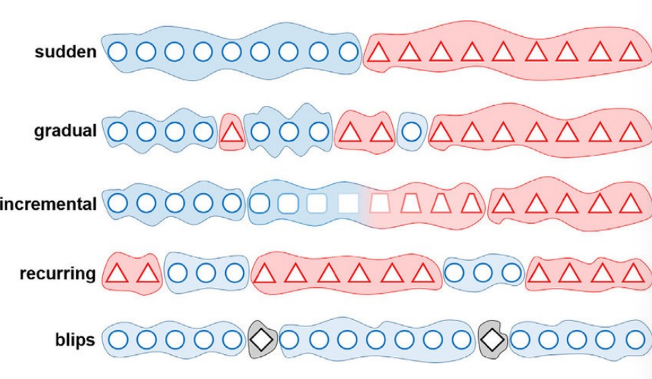
• Concept drift: In most applications, the data distribution changes overtime, for example, the pattern of sales in a given hour throughout the day is not similar to another hour of the day/week/year. This leads to changes in the output of the algorithm as well

Big data - Three V + 4

Big data follows three fundamentals:

1. Volume: defines the huge amount of data produced
2. Variety: refers to the diversity of data types and sources, where most data is unstructured at first, and doesn't seem to contain any relationships, but thanks to big data algorithms, it is able to be examined for relationships
3. Velocity: refers to the speed in which data is generated, analized and reprocessed plus...
4. Validity: is the guarantee of data quality, alternatively Veracity is the authenticity and credibility of the data. Big data involves working with all degrees of quality
5. Value: denotes the added value for a business
6. Variability: taking into consideration the variability of data, it differs from variety as variability is inherited in the single data point, example: "variety is a shop that offers 6 kinds of coffees, variability is a single coffee that tastes differently everyday"
7. Visualization: using big data to create summaries which are easily readable by a person, like charts

Applications

Here are some examples of applications of the different data mining fundamentals

Store product placement

A merchant has a set of $d$ products together with a history of previous transactions, containing the items that were bought by a customer. The merchant would like to know how to place a product on the shelves to increase the likelihood that items that are frequently bought together are placed on adjacent shelves

This problem is closely related to frequent pattern mining to determine groups of items that are frequently bought together

Product recommendations

A merchant has an $n \times d$ binary matrix $D$ representing the buying behaviour of $n$ customer across $d$ items. We assume that this matrix is sparse as customers often buy very few products compared to how many are available. We want to create recommendations to customers.

There are 3 ways to solve this problem:

1. Association rule mining: ?
2. Determine the most similar rows to the target customer, then recommend the most common item which occurs in those similar rows
3. Create a clustering of similar customers, and in each segment, use association pattern mining to make the recommendations